Blog

VectoredIn is a tool I developed to visualize the job market and job postings from LinkedIn utilising various tools and techniques from the NLP and LLM space. To read more about the project, look here.

Data

For this project, I built upon this Kaggle dataset here, which originally contained over 100,000 job postings, and I increased this to just over 1 Million individual job postings.

With each job posting having an average of 500 words (600 tokens) for the description alone, alongside some additional metadata, this is a reasonably large dataset.

The main goal of this project was to use LLM’s to create a vector representation of each individual job posting, and store these in a open-source vector database from Weaviate. The way a classical embedding process works is that you feed in a body of text (Document, Article, Paper, etc.) and you get out a vector representation of the text. This vector represents the semantic meaning behind the text, with similar articles of text being closer to each other in the vector space.

Having to embed over 600 million tokens (if we were simply to feed in each full job posting to the model) is pretty inefficient and costly.

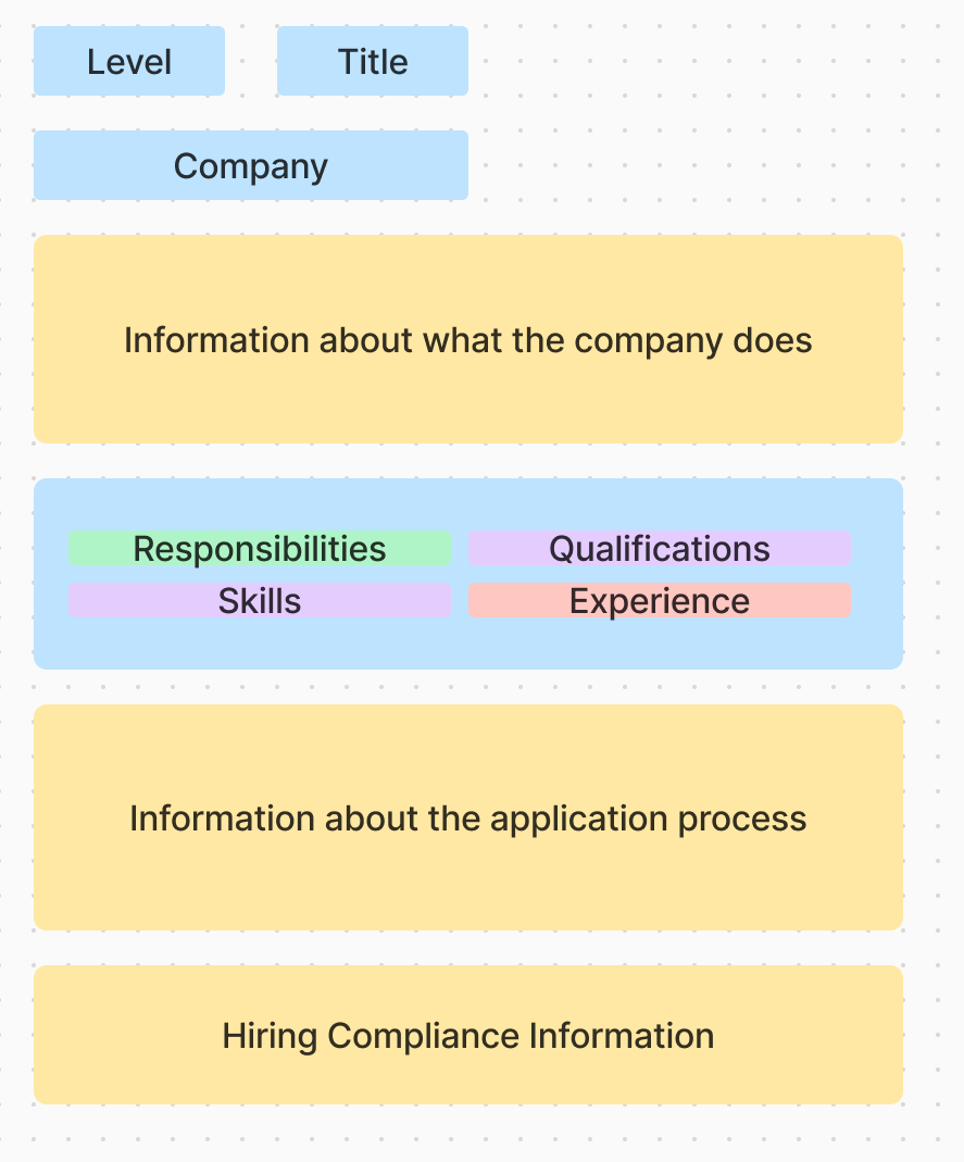
Anatomy of a Job Posting

Job postings are a semi-structured format of data. They are all quite different from each other, but if we zoom out, they all are made up of the same sub-components. We can expect a job posting to have a title, responsibilities, skills, qualifications, and tools, all in varying amounts. This is alongside some additional text, which is not relevant to the actual role, but more contextual to the company and the hiring process.

The diagram here shows roughly what we would expect to see when we are looking at a job posting. With the aim of trying to reduce the amount of data, we can see some text that we can remove, such as general information about the company, the hiring process, and compliance information. While this information may be relevant when applying for a job, it is not relevant to the role itself.

Vector Embedding and Cosine Distance

Let’s go over a quick explainer about the process of creating a vector embedding and how we can use it to compare the similarity between two bodies of text. When we create an embedding of a body of text, we are creating a vector (array of numbers) that represents the semantic meaning behind the text. These vectors don’t contain any meaning by themselves, but they give us the ability to compare the similarity between two bodies of text, by comparing their respective embedding vectors.

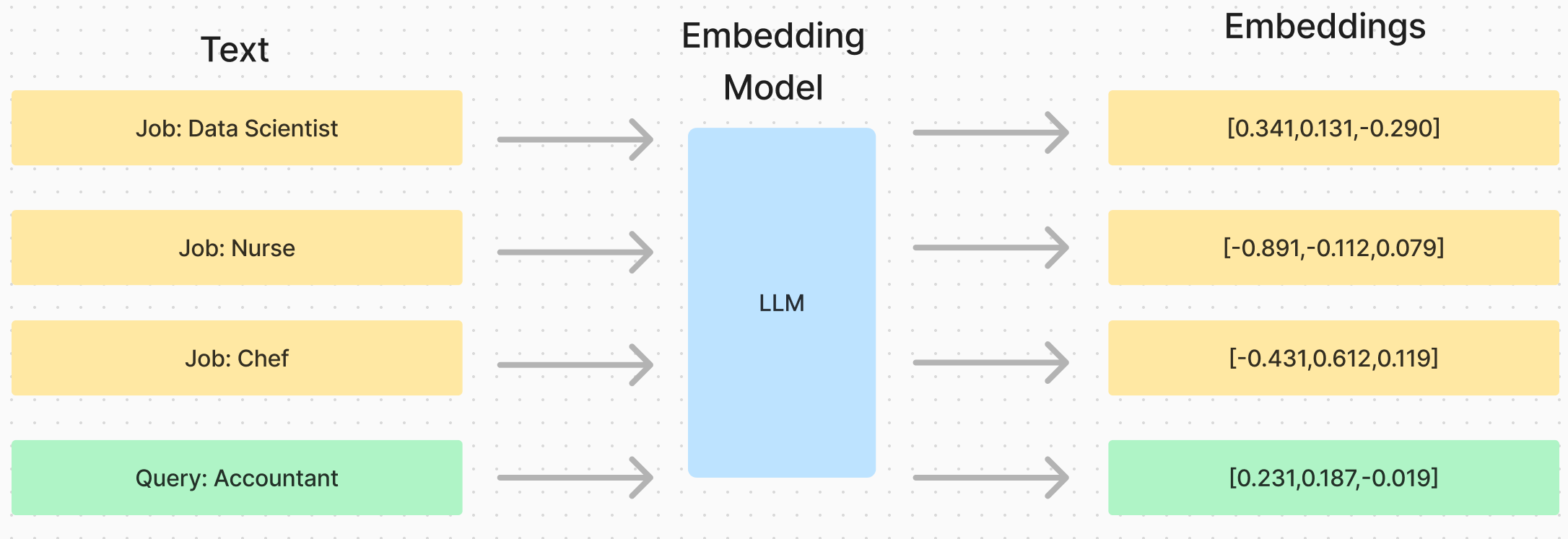
In this example, we’ve created embeddings with a dimensionality of 3, just to provide us with an easy visual representation. In reality, the embedding will be much larger, the actual dimensionality of the embedding we use is 1563, which is a little harder to visualise than 3 dimensions.

In this diagram we have created embedding vectors for a sample of ~300 jobs, and added in 3 queries as embeddings (the job’s we are looking for). The query embeddings are the green diamonds, and the specific job posting we are looking at is highlighted in red.

Here we can see the 3 red lines showing the distance between the queries and the highlighted job posting. This is what we will us as our semantic distance moving forward. To be more accurate, what is actually represented by the red line is the Euclidean Distance between the two points, but in this project we are using the Cosine Distance between the two vectors, but for explanation purposes they represent the same thing.

While this visualisation of embeddings in 3 dimensions is useful for this simple explanation of distance and embeddings, its does not provide much more than that. All further visualisations will be based on the 3 distances between a job postings and the queries, calculated using the Cosine Distance over 1563 dimensional embedding vectors.

Lets look at some of the techniques that we can use to extract key information to create our embedding vectors.

Techniques

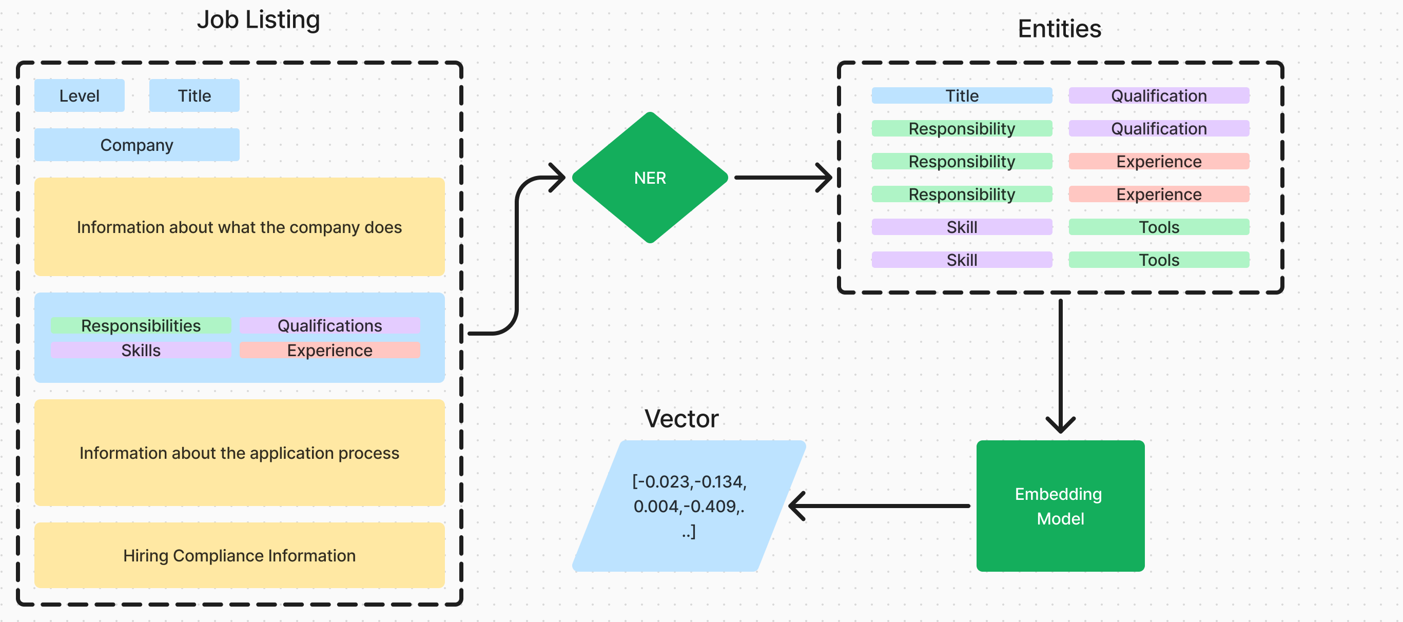
There are several techniques that can be used to extract the key information from a body of text, the most popular being Named Entity Recognition (NER). NER involves training a model, (LLM or in this case a statistical model) to identify and classify named entities in a text. The NER model we have used and finetuned is from the spaCy library, which is a popular NLP library.

NER

To utilise NER in this context, we first have to identify the relevant entity categories we want to extract. Some example of these are: [RESPONSIBILITIES, SKILLS, TOOLS, QUALIFICATIONS]. We then train the model to identify these entities in the text, and classify them into the relevant categories. Building on our diagram from above, this is a representation of how this model works in relation to our goal of reducing the dimensionality of the data.

The benefits of this are twofold:

1. Reducing the amount of data. The data extracted using NER equates to 30% of the original data, which is a significant reduction.
2. Removed unrelated information. We have removed a fair amount of the text that is not pertinent to the underlying role, which should increase the quality of the embeddings.

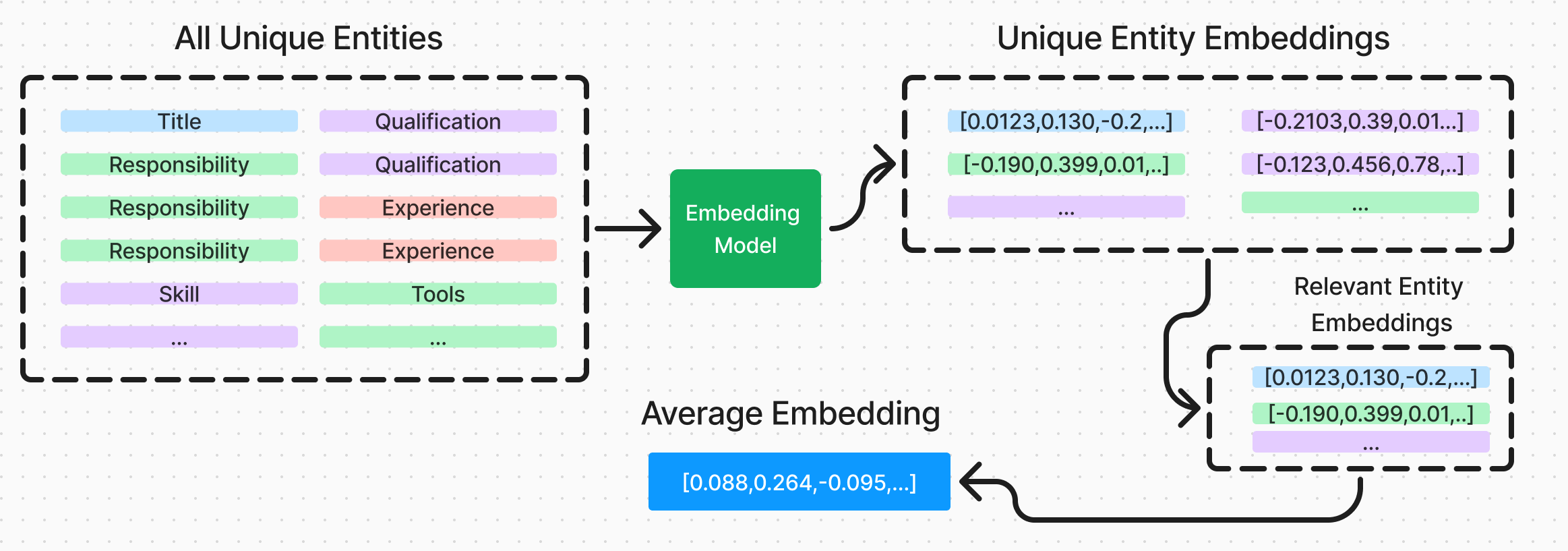
Sub-Component Embedding

Sub-Component Embedding (SCE) builds on our NER technique above, and involves taking the output of the NER model and using it to create a new embedding for each sub component. All these individual embeddings can then be used to create a Composite Embedding Vector (CEV) for the entire job posting. This presents us with three major benefits:

1. Further data reduction. As we now only have to create embeddings for each unique sub-component, we can greatly reduce the amount of data we have to send through a LLM. Alongside this, we have also changed the way this scales with the amount of data, scaling logarithmically.
2. Flexibility. Having the ability to recompile an embedding from a range of sub-components means that we have flexibility in the way we combine the sub-components, whether they are all weighted equally, or a weighted relative to their classification.
3. Visualisation. Having the ability to visualise each sub-component by it’s self, and in relation to the CEV, we can gain an insight into how each of the sub-components relate to the job posting, and the axis we are visualising them on.

Plotting the quantity of tokens required to generate embeddings for each of these methods, we can see the impact of our techniques, and how the sub-component embedding method is the most efficient. At 1 million job postings, embedding the full NER of the job posting uses 30% of the tokens that embedding the full description needs. Further, the sub-component embedding method uses only 6% of the tokens.

Visualisation

One of the main benefits of utilising sub-component embedding is that when we are visualising the semantic distance between each of the sub-components, we can see how they relate to the overall job posting.

In the diagram below, we can see the cosine distances and relationship between each of the individual sub-components and the three axis. Further, we can see how the composite embedding vector relates to each of the sub-components, and the axis.

The first diagram represents a range of job postings and their relative relations to the 3 user defined axis. The point highlighted in red is the job posting we have selected. The second diagram we can see the sub-components of this job posting, and their relative relations to the 3 user defined axis, along with the composite embedding vector of the job posting.

For example we can see that one of the sub-components Experience in data management and automation is more related to the Data Science and Machine Learning Engineer axis, in comparison to the Accountant axis, despite this being a job posting very related to an Accountant role. But the composite embedding takes into account all the sub components, including some very related to the Accountant role, such as Bachelors Degree in Accounting or Business related field. Try hovering on the points above to see how this is represented in the diagram.

An important point to note here, is that while we talk about the Composite Embedding Vector (CEV) as an average of the Sub Component Embeddings (SCE), we do not expect the cosine distance of the CEV to be the average of the cosine distance of the SCEs. This is because the CEV represents a new point in the high-dimensional embedding space that captures the aggregate semantic meaning of all sub-components. All the vectors here are represented in a vector space of 1536 dimensions, from the new OpenAI 'text-embedding-3-small' model.

Compositing Embedding Vectors

As mentioned above, when we are compositing a new vector from SCEs, there are many different methods we can use. The simplest of which would be to take the average of all the SCEs as they are and treat them all equally.

Here’s an example of the SCEs for the job posting we visualised above.

{    
    'embeddings': {
        'company_name': {
            'Deloitte': array([0.0426881, -0.03636974, 0.02759714, ... ])
        },
        'entities_EXPERIENCE': {
            "3+ years' experience in federal partnership tax compliance...": array([-0.0206065, 0.0104712, 0.06552737, ... ]),
            'Experience with data management and automation tools ': array([-0.02074211, 0.02936463, 0.06454881, ... ]),
            'Experience working in a fast-paced, team environment ..': array([-0.05655309, 0.01771902, 0.01467823, ... ])
        },
        'entities_QUALIFICATIONS': {
          'Bachelors degree in accounting or business-related field ': array([-0.02273333, 0.01862575, 0.04938539, ... ]),
        }
        'entities_RESPONSABILITY': {
            'Aptitude in Microsoft Office, especially Microsoft Excel': array([0.01134986, 0.00715933, 0.06455616, ... ]),
            'Lead client engagement teams and client delivery ': array([0.03342095, 0.01799032, 0.10103559, ... ]),
            'Lead the development of new features and ... ': array([0.01359465, -0.00747398, 0.0514259, ... ]),
            'of the current range is $82,880 to $175,500.': array([0.01902576, 0.01339932, 0.09241084, ... ]),
            'provide you with a great work/life fit and ...': array([0.00955491, 0.01953559, 0.04167593, ... ])
        },
        'entities_TOOLS': {
            'Deloitte Tax': array([0.01264361, 0.01308516, 0.03882795, ... ])
        },
        'industry_names': {
            'Accounting': array([-0.02227813, -0.02324294, 0.08319844, ... ]),
            'Business Consulting and Services': array([-0.03887666, 0.00595183, 0.0723723, ... ]),
            'IT Services and IT Consulting': array([-0.04406529, -0.01873075, 0.06618199, ... ])
        },
        'job_functions': {
            'Accounting/Auditing': array([-0.05215971, 0.01514608, 0.04201899, ... ])
        },
        'title': {
            'Tax Senior - PSG - Investment Management Reporting ...': array([-0.02505, 0.04683963, 0.05933352, ... ])
        }
    }
}

Equal Entities

So to achieve the simplest method of composition, we would take the average of all the SCEs, and treat them all equally.

import numpy as np

# Extract all the arrays
all_arrays = []
for category in embeddings.values():
    for embedding in category.values():
        all_arrays.append(embedding)

# Stack the arrays
stacked_arrays = np.stack(all_arrays)

# Calculate the mean
composite_embedding_vector = np.mean(stacked_arrays, axis=0)

Equal Classes

This approach does work and provide reasonable results for examples like this, but what we gain in simplicity here, we lose in performance. While not the case in this example, there is are many job listings where the balance between the categories is very heavily skewed in one direction. For example, a job posting for a Full Stack Developer may only list 3 responsibilities, while listing over 20 tools and frameworks. The CEV from a imbalanced set of entities like this, will not accurately represent the underlying job post. A simple fix for this is to take the average of the SCEs for each category, and then take the average of the resulting vectors to create our CEV.

import numpy as np

# Extract all the arrays
all_cat_means = []
for category in embeddings.values():
    # Extract all the arrays for each category
    category_embeddings = []
    for embedding in category.values():
        category_embeddings.append(embedding)
    # Calculate the mean of the arrays for each category
    category_embedding = np.stack((category_embeddings).mean(axis=0))
    all_cat_means.append(category_embedding)

# Stack the arrays
stacked_arrays = np.stack(all_cat_means)

# Calculate the mean
composite_embedding_vector = np.mean(stacked_arrays, axis=0)

Custom Class Weighting

For the third approach, we can build on our second approach and add in manual weights (or optimized weights) to each of the categories. This is a bit more complex but can be an effective way to get a good balance between the categories. The only important thing to note here is that all the weights need to add up to 1, and not every category is required to be present in every listing.

import numpy as np
weights = {
  title: 5,
  company_name: 1,
  industry_names: 1,
  job_functions: 2.5,
  entities_RESPONSABILITY: 2,
  entities_TOOLS: 2,
  entities_QUALIFICATIONS: 2,
  ...
}

# Extract all the arrays
all_cat_means = []
category_weights = []
for category in embeddings.values():
    # Extract all the arrays for each category
    cateogry_weight = weights[category]
    category_embeddings = []
    for embedding in category.values():
        category_embeddings.append(embedding)
    # Calculate the mean of the arrays for each category
    category_embedding = np.stack((category_embeddings).mean(axis=0))*category_weight
    all_cat_means.append(category_embedding)
    category_weights.append(category_weight)

# Stack the arrays
stacked_arrays = np.stack(all_cat_means)

# Calculate the mean
composite_embedding_vector = np.mean(stacked_arrays, axis=0)/np.sum(category_weights)

The approach we took in this project is the second one, as it gives us a good balance between simplicity and performance. But we will get into a comparison of the different approaches, how they influence the results, and what metrics we can use to evaluate them in the next post.

Evaluation

When comparing how these 3 different approaches, Full Description, Full NER, and SCE, influence the resulting embedding vector, there are two main metrics we can look at. Absolute distance between the same vector across all the approaches, and the relative distance between a set of vectors in one embedding compared to the distance of the same set in another.

1. Absolute distance between the same vector across all the approaches (Cosine Distance):

Let $v_F$, $v_N$, and $v_S$ be the embedding vectors for a job posting using Full Description, Full NER, and SCE approaches respectively. We can calculate the cosine similarity between these vectors:

$$ \text{Similarity}(v_1, v_2) = \cos(\theta) = \frac{v_1 \cdot v_2}{|v_1| |v_2|} $$

We can then compare: $$ \text{Sim}(v_F, v_N), \text{Sim}(v_F, v_S), \text{Sim}(v_N, v_S) $$

2. Relative distance between a set of vectors across all the approaches:

For a set of job postings $J = {j_1, j_2, …, j_n}$, let $V_F$, $V_N$, and $V_S$ be the sets of embedding vectors using Full Description, Full NER, and SCE approaches respectively.

We can compare the pairwise distances within each set:

$$ D_X = {\text{Sim}(v_i, v_j) | v_i, v_j \in V_X, i \neq j} $$

Where $X$ is F, N, or S for each approach.

We can then compare the distributions of $D_F$, $D_N$, and $D_S$ to assess how each approach preserves relative distances between job postings.

These two metrics are related but important for different reasons. The second metric is important for when you are performing any clustering or classification tasks on the resulting vectors using unsupervised learning. You can have a very small relative distance metric, but a large absolute distance metric. However, the reverse is not true, if you have a small absolute distance metric, you must have a low relative distance metric. The absolute distance metric is the more important one for the task we have at hand, due to the fact that we are trying to find the most similar job postings to a given query. That is, we want our job postings to remain in the relative same vector space as much as possible.

It’s important to note here that both of these metrics are relative metrics, and we don’t have a ground truth (correct embedding) to compare them against. In this case we are using the Full Description embedding $v_F$ as a ground truth. While this is sufficient for the moment, as we discussed above in Anatomy of a Job Posting, the full description contains information that is not pertinent to the underlying role, this means that the Full Description may not be the best embedding for the task at hand.

With these two main metrics defined lets compare the results of some of our embedding methods:

These results were generated over a reasonably small subset of 10,000 but should give us a fair idea of the impact the different embedding/compositing methods have on our final result. We’ve added in some less useful vector methods to give us a wider comparison, such as just embedding the title, or the responsibilities, and simply mirroring the original vector. Here we can see that using a custom weight of our cub-component embedding when creating our CEV, we can achieve similar distance metrics to the full NER, again while embedding 5 times less data.

While we talk about these metric and methods here as akin to “performance”, this is only relative performance to the original method, which is embedding the full job posting. So in this case, it would not be fair to draw concrete conclusions about what method is “best” overall, but only to highlight the difference between them and the tradeoff between data efficiency and similarity to the base method. This presents itself as a pretty classical optimization problem, and there are more advanced techniques we will look at in the future.

Further Work

This has been an interesting introduction for myself when exploring the world of vector databases, embedding models, NER and LLMs. However there’s still a lot of improvement that can be made to this method, and the VectoredIn project overall. A few of these areas worth considering are:

• Improving the NER, and changing from spaCy to a finetuned BERT or DistilBERT.
• Optimizing the custom HNSW search algorithm to allow for filtering.
• Exploring more a robust “ground-truth”, apart from comparison to embedding the full listing.
• Two stage preprocessing, grouping very similar entities together to only embed them once.
• Classification, creating classes and classification model to get standardized titles.
• Job fit, being able to retrieve job listings that best match a candidate.
• Overall memory/server optimization, it’s veeery slow.

So if you are interested in any of the above, keep your eyes peeled for updates.

As always, with any questions or insights, you can reach me at nick@nbdata.co

Thanks for reading!